Hydrology and Water Resources

Hydrologic cycle is the continuous movement of water on, above, and below the Earth’s surface. It includes processes such as evaporation, condensation, precipitation, infiltration, runoff, and subsurface flow. For example, when a summer storm drops 20 mm of rain on a watershed, a portion of that water infiltrates into the soil, some becomes surface runoff that feeds streams, and the remainder evaporates back to the atmosphere. Understanding the cycle is essential for predicting water availability, designing storage facilities, and assessing climate change impacts. A major challenge is quantifying each component accurately because they vary spatially and temporally, especially in regions with complex topography or land‑use change.

Watershed (also called a drainage basin or catchment) is an area of land where all precipitation collects and drains to a common outlet, such as a river mouth or lake. Watersheds are the fundamental units for hydrologic analysis because they define the spatial extent of water and pollutant transport. For instance, a 150‑km² watershed feeding a municipal water supply may be divided into sub‑basins for detailed modeling, allowing engineers to identify critical source areas of contamination. Challenges include delineating boundaries in flat terrain, accounting for underground flow paths, and integrating data from disparate sources, such as satellite imagery and field surveys.

Runoff refers to the portion of precipitation that flows over the land surface toward streams and rivers. It is driven by the balance between rainfall intensity, land‑cover characteristics, and soil infiltration capacity. A practical application is the design of storm‑water drainage systems in urban areas, where impervious surfaces increase runoff volumes and peak flows, leading to higher flood risk. Engineers often use the Curve Number method to estimate runoff from land‑use data; however, the method assumes uniform soil properties and may over‑ or underestimate runoff when soils are heterogeneous or when antecedent moisture conditions are extreme.

Infiltration is the process by which water enters the soil matrix from the land surface. It depends on soil texture, structure, organic matter content, and antecedent moisture. In agricultural engineering, enhancing infiltration through practices such as conservation tillage or the installation of infiltration basins can reduce surface runoff and improve groundwater recharge. One challenge is that infiltration rates can decline rapidly during prolonged rainfall events, leading to unexpected runoff generation and potential flooding.

Percolation is the downward movement of water through the unsaturated zone toward the saturated zone. Percolation rates are controlled by hydraulic conductivity and the water content gradient. In managed aquifer recharge projects, engineers inject surface water into infiltration ponds to accelerate percolation, thereby augmenting groundwater supplies. However, the presence of low‑permeability clay layers can impede percolation, causing water to pond on the surface and increasing the risk of surface‑water contamination.

Evapotranspiration (ET) combines evaporation from soil and water bodies with transpiration from plants. ET is a major component of the water balance, especially in arid and semi‑arid regions where it can exceed precipitation. Accurate ET estimation is critical for irrigation scheduling; for example, using reference ET values from the Penman‑Monteith equation allows farmers to determine the amount of water needed to maintain crop yields. The challenge lies in capturing spatial variability of vegetation types, canopy heights, and soil moisture, which often requires remote sensing data and sophisticated models.

Precipitation encompasses all forms of water falling from the atmosphere, including rain, snow, sleet, and hail. Precipitation intensity and duration directly influence runoff generation and flood potential. In mountainous watersheds, snowpack accumulation and melt are key drivers of seasonal streamflow. Engineers use snow‑melt models, such as the degree‑day method, to forecast spring runoff and to design reservoirs that can capture peak flows. Uncertainty in precipitation forecasts, especially under changing climate patterns, remains a significant hurdle for water‑resource planning.

Streamflow is the volume of water moving through a channel per unit time, typically expressed in cubic meters per second (m³ s⁻¹). Continuous streamflow records are essential for calibrating hydrologic models, estimating flood frequencies, and allocating water rights. For example, a downstream city relying on a river for municipal supply may use long‑term flow statistics to negotiate water‑allocation agreements with upstream users. Challenges include maintaining gauge stations in remote locations, dealing with data gaps, and accounting for anthropogenic alterations such as dam operations that modify natural flow regimes.

Baseflow is the portion of streamflow sustained by groundwater discharge during periods without precipitation. Baseflow provides ecological stability by maintaining stream habitats during dry spells. Engineers often separate baseflow from total flow using hydrograph separation techniques to assess the health of aquifer‑stream connections. A difficulty arises when groundwater extraction lowers the water table, reducing baseflow contributions and potentially impairing downstream ecosystems.

Flood occurs when water exceeds the capacity of a channel or storage area, inundating adjacent land. Flood risk assessment involves frequency analysis of peak discharges, mapping of floodplains, and evaluation of potential damages. In urban planning, designers may incorporate levees, floodwalls, and retention basins to mitigate flood impacts. However, climate‑induced changes in precipitation intensity and sea‑level rise can render historical flood data less reliable, challenging the design of resilient infrastructure.

Drought is a prolonged period of deficient water availability, affecting both surface and groundwater resources. Drought indices, such as the Standardized Precipitation Index (SPI), help quantify severity and duration. Water managers may implement drought contingency plans that include water‑use restrictions, supplemental pumping, and the activation of emergency water‑transfer agreements. The unpredictability of drought onset and the competing demands of agriculture, industry, and domestic users make drought management a complex, multi‑objective problem.

Groundwater is water stored in the saturated zones of soils and rocks beneath the Earth’s surface. It supplies a significant portion of drinking water worldwide, especially in regions lacking surface‑water infrastructure. Groundwater extraction is governed by the principle of sustainable yield, which requires that withdrawal rates not exceed natural recharge over the long term. Over‑pumping can lead to problems such as land subsidence, reduced streamflow, and saltwater intrusion in coastal aquifers. Managing these challenges demands accurate aquifer characterization and robust monitoring networks.

Aquifer is a geologic formation capable of storing and transmitting groundwater. Aquifers are classified as confined, unconfined, or semi‑confined based on hydraulic boundaries. For example, a confined aquifer overlain by an impermeable aquitard may be tapped by a well that yields high pressure, enabling artesian flow. Aquifer heterogeneity, such as the presence of low‑permeability lenses, can create preferential flow paths that complicate groundwater modeling and the prediction of contaminant migration.

Recharge denotes the process by which water enters an aquifer, replenishing its storage. Natural recharge occurs through infiltration of precipitation, river leakage, and seepage from lakes. Artificial recharge techniques, such as injection wells and surface spreading basins, are employed to augment groundwater supplies in water‑scarce regions. The effectiveness of recharge projects depends on soil permeability, hydraulic connectivity, and the quality of the recharging water; contaminants introduced during recharge can degrade aquifer water quality.

Discharge is the volume of water leaving an aquifer or surface‑water system, expressed as a flow rate. In groundwater studies, discharge is often measured at springs or wells and used to estimate aquifer hydraulic properties. In surface‑water contexts, discharge at a gauging station provides information on river health, flood risk, and water‑resource allocation. Determining accurate discharge values can be difficult when flow is highly variable, when channel geometry changes over time, or when measurement equipment is limited.

Hydraulic conductivity (K) quantifies a material’s ability to transmit water under a hydraulic gradient. It is measured in meters per second (m s⁻¹) and varies widely among geologic media, from 10⁻⁸ m s⁻¹ in clays to 10⁻² m s⁻¹ in gravels. Laboratory tests, such as the constant‑head permeameter, and field tests, such as slug and pumping tests, are used to determine K. Accurate K values are critical for groundwater flow modeling; however, spatial variability and anisotropy often require detailed site investigations and geostatistical interpolation.

Porosity is the fraction of a rock or soil’s volume that consists of void space, expressed as a percentage. Total porosity includes both effective and ineffective pores; effective porosity represents the interconnected voids that contribute to fluid flow. For instance, a sandstone may have a total porosity of 30 % but an effective porosity of 20 % due to isolated pores. Determining effective porosity is essential for estimating groundwater storage and contaminant transport, yet it can be challenging to measure directly in the field.

Specific yield (Sy) is the volume of water that can be drained by gravity from a saturated porous medium per unit surface area, expressed as a dimensionless ratio. It approximates the effective porosity for unconfined aquifers. A high Sy, such as 0.25 for a coarse sand, indicates that a large portion of the stored water can be readily extracted. In contrast, low‑Sy materials, like clays, release water slowly, affecting well performance and recharge rates. Accurate Sy values are needed for water‑budget calculations but are often estimated from field tests with inherent uncertainties.

Transmissivity (T) combines hydraulic conductivity and aquifer thickness to describe the ability of an aquifer to transmit water horizontally. It is expressed in square meters per day (m² d⁻¹). In well‑test analysis, transmissivity is derived from the slope of the drawdown curve. High‑transmissivity aquifers, such as karst limestone, can supply large volumes of water to wells, whereas low‑transmissivity formations limit extraction rates. Estimating T accurately requires reliable K measurements and knowledge of aquifer geometry, which can be complex in heterogeneous settings.

Water table is the upper surface of the saturated zone where pore pressure equals atmospheric pressure. It fluctuates seasonally in response to recharge and discharge processes. Mapping the water‑table elevation using observation wells provides insight into groundwater flow direction and potential for surface‑water interaction. In areas with shallow water tables, capillary rise can affect soil moisture and plant growth, while deep water tables may limit the feasibility of shallow wells. Accurate mapping is hindered by sparse well networks and measurement errors.

Phreatic zone is synonymous with the saturated zone below the water table. It is the region where all voids are filled with water, allowing free movement of groundwater. In engineering practice, the depth of the phreatic zone influences the design of foundations, retaining walls, and underground structures. For example, a deep foundation may need to be extended below the phreatic zone to avoid buoyant forces. Changes in the phreatic zone due to seasonal recharge can alter stability conditions, requiring adaptive design strategies.

Unsaturated zone (vadose zone) lies between the land surface and the water table, containing both air and water. Water movement in the unsaturated zone is governed by capillary forces and moisture gradients, described by Richards’ equation. Understanding unsaturated flow is vital for predicting infiltration, contaminant transport, and the effectiveness of remediation techniques such as soil vapor extraction. The nonlinear nature of unsaturated flow and the difficulty of measuring moisture content in situ make modeling this zone challenging.

Hydraulic gradient (i) is the change in hydraulic head per unit distance, driving groundwater flow according to Darcy’s law. It is dimensionless and often expressed as a slope (e.g., 0.001). A steep hydraulic gradient indicates rapid flow, which can increase the spread of contaminants. In engineering design, hydraulic gradients are used to size drainage pipes, estimate seepage velocities, and assess the stability of earth structures. Accurately measuring gradients requires precise head readings at multiple points, which can be logistically demanding.

Darcy’s law provides the fundamental relationship for laminar flow through porous media: Q = K A i, where Q is discharge, K is hydraulic conductivity, A is cross‑sectional area, and i is hydraulic gradient. It underpins most groundwater flow calculations and modeling efforts. However, Darcy’s law assumes linear, laminar flow and may not hold in fractured rock, high‑velocity conditions, or when preferential pathways dominate. Engineers must verify the applicability of Darcy’s law before using it for design or prediction.

Flow net is a graphical representation of equipotential lines and flow lines used to analyze seepage through earth dams, sheet piles, and foundations. By constructing a flow net, engineers can estimate seepage discharge, hydraulic gradients, and potential zones of piping. The method requires careful placement of lines to satisfy boundary conditions and maintain equal spacing. In complex geometries, creating an accurate flow net can be time‑consuming, and numerical modeling may be preferred for higher precision.

Seepage refers to the slow movement of water through soil or rock, often observed as a gradual discharge from embankments or foundations. Seepage can cause internal erosion, known as piping, which may lead to structural failure. Monitoring seepage rates with weirs or piezometers helps assess dam safety. Mitigation measures include installing cutoff walls, drainage blankets, and toe drains. Predicting seepage accurately is difficult because it depends on soil heterogeneity, anisotropy, and the presence of cracks.

Seepage velocity (v) is the average velocity of water particles moving through the pores of a porous medium, calculated as v = q / n_e, where q is Darcy flux and n_e is effective porosity. Seepage velocity is typically higher than Darcy flux because water moves only through the connected pores. In contaminant transport studies, seepage velocity determines the travel time of pollutants. Estimating n_e accurately is essential, yet field measurements often have high uncertainty, leading to variability in predicted velocities.

Hydraulic radius (R) is the cross‑sectional area of flow divided by the wetted perimeter, used in the Manning equation to compute open‑channel flow. A larger hydraulic radius indicates more efficient flow. In channel design, engineers adjust cross‑sectional shape to increase R and reduce required channel width, thereby minimizing land acquisition costs. However, natural channels often have irregular shapes, making the calculation of R less straightforward and requiring detailed surveying.

Manning’s equation (V = (1/n) R^(2/3) S^(1/2)) relates mean flow velocity (V) to hydraulic radius (R), channel slope (S), and Manning’s roughness coefficient (n). It is widely used for designing culverts, spillways, and irrigation canals. Selecting an appropriate n value is critical; for example, a smooth concrete channel may have n ≈ 0.012, whereas a vegetated floodplain may have n ≈ 0.035. In practice, determining n involves field observations, laboratory tests, or consulting published tables, but site‑specific conditions such as debris accumulation can cause n to change over time.

Roughness coefficient (n) quantifies the resistance to flow caused by channel surface texture, vegetation, and irregularities. It directly influences flow capacity and water‑surface elevations. In flood‑routing models, an inaccurate n can lead to erroneous predictions of peak stage and timing, potentially compromising flood‑risk assessments. Engineers often calibrate n using observed flow data, but the presence of sediment transport, seasonal vegetation growth, and bio‑film formation introduces variability that must be accounted for in long‑term designs.

Flow regime describes the character of fluid motion, ranging from laminar (smooth, orderly) to turbulent (chaotic, mixing). The Reynolds number (Re) determines the regime: Re < 2000 indicates laminar flow, while Re > 4000 suggests turbulent flow. In pipe design, laminar flow results in lower friction losses, whereas turbulent flow increases energy dissipation. Transition zones can be sensitive to surface roughness and pipe diameter. Selecting appropriate pipe materials and diameters helps maintain desired flow regimes and optimize hydraulic efficiency.

Laminar flow is characterized by smooth, parallel layers of fluid with minimal mixing. In small‑diameter pipes or low‑velocity conditions, laminar flow dominates and can be described by the Hagen‑Poiseuille equation. For water‑distribution networks, laminar flow reduces head loss, allowing for smaller pump capacities. However, achieving laminar flow in large‑scale conveyance systems is rarely practical, and designers must anticipate turbulent conditions for most municipal applications.

Turbulent flow exhibits chaotic fluctuations, eddies, and increased mixing, leading to higher friction losses. In open channels, turbulent flow promotes uniform velocity distribution and enhances sediment transport capacity. Engineers use empirical formulas, such as the Darcy‑Weisbach equation with a turbulent friction factor, to estimate head loss. Turbulence intensity can be mitigated by smoothing channel surfaces, but excessive smoothing may reduce habitat diversity in ecological contexts, creating a trade‑off between hydraulic efficiency and environmental considerations.

Reynolds number (Re) is a dimensionless quantity defined as Re = ρ V D / μ, where ρ is fluid density, V is velocity, D is characteristic length (e.g., pipe diameter), and μ is dynamic viscosity. It provides a criterion for predicting flow regime transitions. In hydraulic design, calculating Re helps select appropriate loss‑coefficient correlations and informs scaling of laboratory experiments to field conditions. High variability in water temperature, which affects viscosity, can shift Re values and alter flow regime predictions.

Water balance (or water budget) is an accounting of all inflows, outflows, and storage changes within a defined system over a specified period. The basic equation is P + I = E + R + ΔS, where P is precipitation, I is inflow, E is evapotranspiration, R is runoff, and ΔS is change in storage. Water‑balance analysis is used for watershed planning, reservoir operation, and sustainability assessments. Challenges arise from uncertainties in each term, especially evapotranspiration estimates and groundwater fluxes, which can lead to significant errors in the overall budget.

Mass balance extends the water‑balance concept to include solutes, sediments, or energy, tracking inputs, outputs, and transformations. For contaminant transport, the mass‑balance equation incorporates advection, dispersion, sorption, and degradation processes. Engineers apply mass‑balance calculations to design treatment systems, predict pollutant plume migration, and evaluate remediation effectiveness. Accurate mass‑balance modeling requires reliable parameter values, such as decay constants and sorption coefficients, which are often site‑specific and difficult to obtain.

Water quality refers to the chemical, physical, and biological characteristics of water relative to its intended use. Parameters include temperature, pH, dissolved oxygen, turbidity, nutrients, and contaminants. Water‑quality monitoring informs compliance with regulatory standards, guides treatment plant design, and assesses ecosystem health. For example, elevated nitrate concentrations in agricultural runoff can cause eutrophication in downstream lakes. Managing water quality involves source‑control measures, treatment technologies, and continuous monitoring, all of which face challenges related to detection limits, temporal variability, and emerging pollutants.

Pollutant load is the mass of a contaminant transported by water per unit time, typically expressed in kilograms per day. Load calculations combine concentration data with flow measurements (Load = C × Q). In watershed management, estimating pollutant loads from point and non‑point sources helps prioritize mitigation efforts. A common challenge is the high spatial and temporal variability of non‑point source loads, which require extensive sampling and statistical analysis to quantify accurately.

Sediment transport involves the movement of particulate material by water flow. It is governed by sediment size, flow velocity, turbulence, and channel geometry. The Shields parameter and the Rouse number are commonly used to predict initiation of motion and suspension. In river engineering, sediment transport analysis guides the design of stabilisation measures such as riprap, groynes, and channel realignment. Excessive sedimentation can reduce reservoir capacity, while sediment starvation downstream can cause channel incision and habitat loss. Balancing these effects requires integrated sediment management strategies.

Erosion is the detachment, transport, and deposition of soil particles caused by water flow. Factors influencing erosion include rainfall intensity, slope steepness, soil erodibility, and land cover. The Universal Soil Loss Equation (USLE) estimates average annual soil loss, providing a basis for conservation planning. Practically, engineers implement erosion control measures like contour farming, terracing, and vegetative buffer strips to reduce sediment yield. Predicting erosion rates remains difficult due to the stochastic nature of storm events and the heterogeneity of soil properties.

Deposition occurs when transported sediments settle out of the flow as velocity decreases. Deposition zones, such as river bends and floodplains, can form beneficial habitats but also lead to reduced channel capacity and increased flood risk. In reservoir design, sediment deposition reduces storage over time, necessitating sediment‑management plans such as dredging or flushing operations. Accurately forecasting deposition patterns requires detailed hydraulic and sediment‑transport modeling, which can be computationally intensive.

Scour is the removal of bed or bank material by flowing water, often occurring around hydraulic structures like bridge piers, abutments, and culverts. Scour depth depends on flow velocity, turbulence, sediment size, and foundation geometry. Engineers use empirical formulas, such as the HEC‑18 equations, to estimate potential scour and design protective measures like riprap, collars, or deep foundations. Scour is a leading cause of bridge failure, and its prediction is complicated by fluctuating flow conditions, debris impact, and local hydraulic complexities.

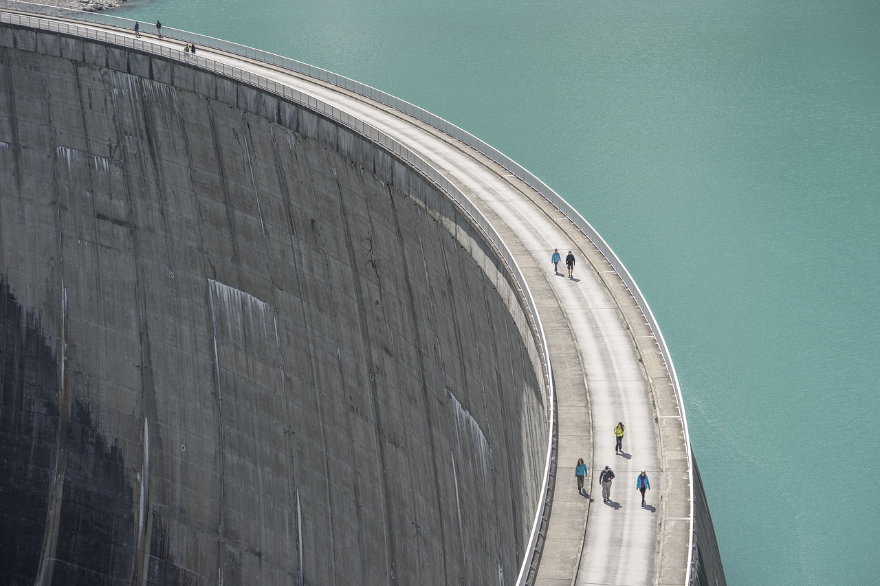
Hydraulic structures encompass dams, weirs, spillways, gates, and related facilities that control water flow for purposes such as flood control, water supply, and hydroelectric power. Proper design requires knowledge of hydraulic principles, structural mechanics, and environmental considerations. For instance, a spillway must safely convey design flood discharges without overtopping the dam, while a weir can be used to measure flow rates. Challenges include accommodating extreme events, sediment passage, and fish migration, all of which may require adaptive or multi‑purpose designs.

Dam is a barrier that impounds water for storage, power generation, or flood control. Dams are classified by type (e.g., gravity, arch, embankment) and function. Design considerations include foundation conditions, seismic loading, seepage control, and spillway capacity. The failure of a dam can have catastrophic consequences, as illustrated by historical events. Modern dam safety programs incorporate regular inspections, instrumentation, and emergency action plans to mitigate risks. Balancing water‑resource benefits with environmental and social impacts remains a central challenge.

Reservoir is the artificial lake created behind a dam, serving as a storage facility for water supply, irrigation, recreation, and hydroelectric generation. Reservoir operation involves balancing inflow forecasts, demand schedules, and flood‑mitigation objectives. Seasonal drawdown may expose shoreline, affecting habitat and water quality. Sedimentation progressively reduces reservoir capacity, prompting the need for sediment‑management strategies such as upstream check dams, sediment bypass tunnels, or periodic dredging. Predicting long‑term storage loss requires integrating watershed erosion models with reservoir sedimentation calculations.

Spillway provides a controlled pathway for excess water to bypass a dam, protecting the structure from overtopping. Spillways can be overflow, gated, or siphon types, each with distinct hydraulic characteristics. Designing a spillway involves calculating the design flood discharge, estimating hydraulic head, and ensuring structural stability against cavitation and erosion. In high‑head designs, aeration devices are installed to prevent vacuum formation. Spillway capacity must accommodate changing climate patterns, which may increase the frequency of extreme rainfall events beyond historical design criteria.

Weir is a low‑profile barrier across an open channel used to measure flow or regulate water level. Common types include sharp‑crested, broad‑crested, and V‑notched weirs. The discharge equation for a sharp‑crested weir is Q = C L H^(3/2), where C is the discharge coefficient, L is the crest length, and H is the head over the crest. Accurate flow measurement requires proper installation, regular cleaning to remove debris, and calibration of C values. Errors can arise from submergence, downstream conditions, and surface tension effects, especially for small‑scale weirs.

Outlet works consist of gates, valves, and conduits that regulate the release of water from a reservoir or canal. They enable precise control of downstream flows for water‑supply, ecological, or flood‑mitigation purposes. The design of outlet works includes considerations of hydraulic capacity, structural strength, and operational reliability. For example, a sluice gate may be sized to pass the design flood while allowing fine adjustments during normal operation. Maintenance challenges include corrosion, sediment clogging, and mechanical wear, which can impair functionality if not addressed.

Sluice gate is a movable barrier that slides vertically or horizontally to control water discharge. Sluice gates are commonly used in irrigation canals, dam outlets, and flood‑control structures. Their operation can be manual, hydraulic, or electric, with automation enabling rapid response to changing flow conditions. Designing a sluice gate involves calculating the required opening size, structural loads, and sealing mechanisms to prevent leakage. Failure modes such as gate sticking or hinge corrosion must be mitigated through regular inspection and preventive maintenance.

Canal is an artificial waterway constructed for conveyance of water for irrigation, navigation, or drainage. Canal design considers alignment, cross‑sectional shape, lining material, and hydraulic capacity. Lined canals reduce seepage losses and improve conveyance efficiency, while unlined canals may be more economical but suffer from higher water loss and weed growth. Hydraulic calculations determine the appropriate slope and roughness coefficient to achieve desired discharge. In arid regions, canal evaporation can be a significant water loss, prompting the use of covered or underground conduits as mitigation measures.

Irrigation involves the artificial application of water to land to support agricultural production. Irrigation methods range from surface flooding to pressurized sprinkler and drip systems. Selecting an appropriate method depends on crop type, soil characteristics, water availability, and energy costs. For example, drip irrigation delivers water directly to the root zone, reducing evaporation losses and improving water‑use efficiency. However, it requires precise design of emitters, pressure regulation, and maintenance to prevent clogging. Balancing water‑conservation goals with crop‑yield requirements remains a central challenge in irrigation engineering.

Drainage removes excess water from soils or surface water bodies to improve land productivity, prevent water‑logging, and protect infrastructure. Drainage systems include surface ditches, subsurface tile lines, and pumped wells. Designing a drainage network involves determining the drainage coefficient, spacing of ditches, and hydraulic conductivity of the soil. In coastal areas, drainage must also consider sea‑level rise and saltwater intrusion, which can compromise the effectiveness of freshwater removal. Proper drainage design mitigates the risk of soil salinization, reduces greenhouse‑gas emissions from anaerobic soils, and enhances crop yields.

Water rights are legal entitlements that allocate water among users based on statutory, prior‑appropriation, or riparian principles. Understanding water‑right frameworks is essential for engineers involved in allocation studies, permit applications, and conflict resolution. For instance, a senior water‑right holder may have priority access during drought, limiting the water available for junior users. Complexities arise when multiple jurisdictions overlap, when environmental flow requirements are imposed, or when climate change alters water availability, necessitating adaptive management and renegotiation of rights.

Allocation describes the distribution of available water among competing users, such as agriculture, industry, domestic supply, and the environment. Allocation models integrate hydrologic forecasts, demand projections, and legal constraints to optimize water‑use efficiency. Practical tools include linear programming, game theory, and simulation‑based approaches. A common challenge is ensuring equity while meeting reliability targets, especially under uncertain climate scenarios that may reduce overall water availability. Stakeholder engagement and transparent decision‑making processes are critical for successful allocation outcomes.

Conjunctive use combines surface‑water and groundwater resources to improve reliability and sustainability. For example, a municipal system may draw from a reservoir during wet periods and supplement supply with groundwater pumping during drought. This approach can also enhance groundwater recharge by releasing surface water into infiltration basins during high‑flow events. Managing conjunctive use requires careful monitoring of aquifer levels, water‑quality interactions, and the impact of pumping on stream baseflow. Over‑extraction can lead to declining water tables and land subsidence, undermining the benefits of the strategy.

Water supply systems deliver potable water from source to consumer through a network of treatment plants, storage facilities, and distribution pipelines. Design considerations include source reliability, treatment technology, pipe sizing, and pressure management. For instance, a city may employ a multi‑stage treatment train incorporating coagulation, filtration, and disinfection to meet health standards. Challenges encompass aging infrastructure, leak detection, and maintaining water quality during storage. Advanced monitoring, real‑time pressure control, and asset management programs are employed to address these issues.

Demand forecasting predicts future water consumption patterns based on population growth, economic development, and climate factors. Accurate forecasts guide capacity planning for treatment plants, reservoirs, and distribution networks. Methods range from simple extrapolation to sophisticated econometric models that incorporate price elasticity, conservation measures, and behavioral changes. Uncertainty in forecasts can lead to over‑building, resulting in unnecessary capital expenditures, or under‑building, causing supply shortages. Incorporating scenario analysis and adaptive management helps mitigate these risks.

Climate change impacts on water resources include altered precipitation regimes, increased temperature, and more frequent extreme events. Hydrologic models are updated with downscaled climate projections to assess changes in streamflow, groundwater recharge, and water‑quality trends. For example, a basin may experience a shift from snow‑melt‑dominated runoff to rain‑dominant runoff, affecting reservoir operation and flood risk. Engineers must design flexible infrastructure capable of accommodating a wide range of future conditions, often requiring higher safety factors and adaptive operating rules.

Remote sensing provides spatially extensive data on land surface characteristics, precipitation, snow cover, and vegetation health. Satellite sensors such as MODIS, Landsat, and Sentinel deliver observations that support hydrologic modeling, flood mapping, and drought monitoring. For instance, radar‑derived rainfall estimates can supplement ground gauge networks in remote regions. Limitations include sensor resolution, cloud contamination, and the need for ground truth validation. Integrating remote‑sensing products with in‑situ measurements improves model accuracy and situational awareness during emergencies.

GIS (Geographic Information System) enables the storage, analysis, and visualization of spatial data related to water resources. GIS tools are used to delineate watersheds, map land‑use changes, and generate hydraulic models. By linking hydrologic data with demographic and infrastructure layers, planners can assess vulnerability, prioritize investments, and communicate findings to stakeholders. Data quality, projection inconsistencies, and the integration of heterogeneous datasets pose challenges that require careful data management and validation.

Hydrologic modeling simulates the movement of water through the hydrologic cycle using mathematical representations of physical processes. Models range from simple empirical relationships to complex physically‑based distributed simulations. Common applications include flood forecasting, water‑resource allocation, and climate‑impact assessments. Model selection depends on data availability, scale, and purpose. Calibration against observed data is essential to ensure reliability, and sensitivity analysis identifies influential parameters. Model uncertainty must be quantified to inform risk‑based decision making.

Rainfall‑runoff models transform precipitation inputs into runoff estimates, accounting for infiltration, storage, and routing. The SCS Curve Number method, for example, uses land‑use and soil‑type data to estimate runoff depth. More advanced models, such as HEC‑HMS, incorporate event‑based or continuous simulation, sub‑basin routing, and reservoir operation. Accurate rainfall input, appropriate parameterization, and consideration of antecedent moisture conditions are critical for reliable predictions. Model limitations include simplifications of complex processes and the need for extensive calibration data.

Unit hydrograph represents the watershed response to a unit pulse of rainfall excess, providing a basis for linear superposition of multiple storm events. The synthetic unit hydrograph, such as the SCS UH, employs watershed characteristics to generate a hydrograph shape. Engineers use unit hydrographs to develop flood forecasts and design hydraulic structures. Non‑linear watershed behavior, such as saturation excess or threshold effects, can reduce the applicability of the linear unit‑hydrograph concept, requiring alternative modeling approaches.

HEC‑HMS (Hydrologic Engineering Center – Hydrologic Modeling System) is a widely used software for simulating rainfall‑runoff processes, reservoir operations, and channel routing. It supports both event‑based and continuous simulations, allowing users to integrate climate data, land‑use changes, and water‑management decisions. HEC‑HMS outputs are often linked to hydraulic models like HEC‑RAS for floodplain analysis. Effective use of HEC‑HMS requires careful basin delineation, parameter selection, and rigorous calibration and validation against observed streamflow.

HEC‑RAS (River Analysis System) is a hydraulic modeling tool that simulates one‑dimensional water flow in rivers and channels, including flood‑inundation mapping. By inputting geometry, roughness, and flow data, engineers can predict water‑surface elevations, assess flood risk, and evaluate mitigation measures such as levees or floodwalls. Coupling HEC‑RAS with GIS enables rapid generation of floodplain maps for emergency management. Limitations include the assumption of one‑dimensional flow, which may not capture complex three‑dimensional phenomena in wide or highly braided rivers.

MODFLOW is a modular finite‑difference groundwater flow model developed by the USGS. It simulates three‑dimensional subsurface flow, incorporating features such as variable hydraulic properties, stress periods, and boundary conditions. MODFLOW is the foundation for many groundwater‑management studies, including aquifer testing, contaminant transport, and conjunctive‑use analyses. Extensions such as MT3DMS add solute transport capabilities. Successful application requires accurate parameterization, grid discretization, and calibration to observed hydraulic heads and fluxes.

SWAT (Soil and Water Assessment Tool) is a distributed, process‑based model that predicts the impact of land‑use and climate changes on water quantity and quality in large watersheds. SWAT simulates surface runoff, evapotranspiration, groundwater flow, and nutrient cycling. It is employed for evaluating best‑management practices, assessing sediment and pesticide loads, and supporting watershed‑restoration planning. Model complexity demands comprehensive input data, including soils, weather, topography, and management practices, and extensive calibration to observed streamflow and water‑quality data.

Calibration adjusts model parameters to achieve agreement between simulated and observed data, improving predictive capability. Calibration techniques range from manual trial‑and‑error to automated optimization algorithms such as the Shuffled Complex Evolution (SCE